4 R Coding Fundamentals
Now that we’re comfortable with R Studio and have some definitions under our belt, let’s dive in a little into some R code and discuss it. These fundamentals can always be referred back to when we might be stuck coding later on.
4.1 Entering Input
In the R Script area, we write code. Whenever we want to assign a variable, we do so using the assignment operator. The <- symbol is the assignment operator. We can also use = which is a bit more intuitive. It is alright to interchange these when assigning variables.
val <- 1
print(val)
## [1] 1val## [1] 1msg <- "hello"val and msg are both variables that we assigned.
We use the # character to write comments inside our code. Commented code is NOT executed by R.
x <- ## Incomplete expressionAnything to the right of the # (including the # itself) is ignored.
4.2 Running Code
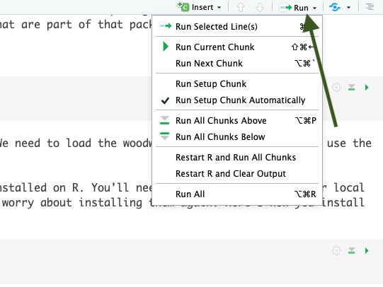
After placing the above code in your R Script area, we can run the code. Code execution is done in the R Console. We can “send” our code in the R Script to the R Console using the Run Button, ctrl + enter (Windows), or cmd + enter (Mac). We can select specific lines of code to run, larger chunks, or the entire R Script.
4.3 Evaluation
When a complete expression is entered at the prompt, it is evaluated and the result of the evaluated expression is returned. The result may be auto-printed.
val <- 14   ## nothing printed
val         ## auto-printing occurs
## [1] 14print(val) ## explicit printing## [1] 14The [1] shown in the output indicates that x is a vector and 14
is its first element. Typically we do not explicitly print variables since auto-printing is easier.
When an R vector is printed you will notice that an index for the
vector is printed in square brackets [] on the side. For example,
see this integer sequence of length 10.
my_seq <- 10:20
my_seq
## [1] 10 11 12 13 14 15 16 17 18 19 20Notice the [1] that preceeds the sequence. The output inside the square bracket is not part of the vector itself, it’s just part of the printed output that has additional information to be more user-friendly. This extra information is not part of the object itself. Also note that we used the : operator to create a sequence of integers from 10 to 20 (10:20).
Note that the : operator is used to create integer sequences.
4.4 R Objects
R has five basic or “atomic” classes of objects:
character
numeric (real numbers)
integer
complex
logical (True/False)
The most basic type of R object is a vector. Empty vectors can be
created with the vector() function. There is really only one rule
about vectors in R, which is that A vector can only contain objects
of the same class.
But of course, like any good rule, there is an exception, which is a list, which we will get to a bit later. A list is represented as a vector but can contain objects of different classes. Indeed, that’s usually why we use them.
4.5 Numbers
Numbers in R are generally treated as numeric objects. We can explicitly declare numbers as integers, floats, etc., but I won’t cover that here.
There is also a special number Inf which represents infinity. This
allows us to represent entities like 1 / 0. This way, Inf can be
used in ordinary calculations; e.g. 1 / Inf is 0.
The value NaN represents an undefined value (“not a number”); e.g. 0
/ 0; NaN can also be thought of as a missing value (more on that
later)
4.6 Attributes
R objects can have attributes, which are like metadata for the object. These metadata can be very useful in that they help to describe the object. For example, column names on a data frame help to tell us what data are contained in each of the columns. Some examples of R object attributes are
names, dimnames
dimensions (e.g. matrices, arrays)
class (e.g. integer, numeric)
length
other user-defined attributes/metadata
Attributes of an object (if any) can be accessed using the
attributes() function. Not all R objects contain attributes, in
which case the attributes() function returns NULL.
4.7 Creating Vectors
The c() function is referred to as the concatenate function. Using this, we can create vectors of objects by concatenating them together.
x <- c(1.25, 2.50)       ## numeric
x <- c(TRUE, FALSE)    ## logical
x <- c(T, F)           ## logical
x <- c("yes", "no", "maybe")  ## character
x <- 25:44              ## integer
x <- c(1+2i, 3+8i)     ## complex
Note that in the above example, T and F are short-hand ways to
specify TRUE and FALSE. However, in general one should try to use
the explicit TRUE and FALSE values when indicating logical
values.
4.8 Mixing Objects
There are occasions when different classes of R objects get mixed together. Sometimes this happens by accident but it can also happen on purpose. So what happens with the following code?
y <- c(1.7, "a")   ## character
y <- c(TRUE, 2)    ## numeric
y <- c("a", TRUE)  ## character
In each case above, we are mixing objects of two different classes in a vector. But remember that the only rule about vectors says this is not allowed. When different objects are mixed in a vector, coercion occurs so that every element in the vector is of the same class.
In the example above, we see the effect of implicit coercion. What R tries to do is find a way to represent all of the objects in the vector in a reasonable fashion. Sometimes this does exactly what you want and…sometimes not. For example, combining a numeric object with a character object will create a character vector, because numbers can usually be easily represented as strings.
4.9 Explicit Coercion
Objects can be explicitly coerced from one class to another using the
as.* functions, if available.
x <- 0:10
class(x)
## [1] "integer"as.numeric(x)## [1] 0 1 2 3 4 5 6 7 8 9 10as.logical(x)## [1] FALSE TRUE TRUE TRUE TRUE TRUE TRUE TRUE TRUE TRUE TRUEas.character(x)## [1] "0" "1" "2" "3" "4" "5" "6" "7" "8" "9" "10"Sometimes, R can’t figure out how to coerce an object and this can
result in NAs being produced.
x <- c("a", "b", "c")
as.numeric(x)
## Warning: NAs introduced by coercion## [1] NA NA NAas.logical(x)## [1] NA NA NAas.complex(x)## Warning: NAs introduced by coercion## [1] NA NA NAWhen nonsensical coercion takes place, you will usually get a warning from R.
4.10 Matrices
Matrices are vectors with a dimension attribute. The dimension attribute is itself an integer vector of length 2 (number of rows, number of columns)
m <- matrix(nrow = 2, ncol = 3)
m
## [,1] [,2] [,3]
## [1,] NA NA NA
## [2,] NA NA NAdim(m)## [1] 2 3attributes(m)## $dim
## [1] 2 3Matrices are constructed column-wise, so entries can be thought of starting in the “upper left” corner and running down the columns.
m <- matrix(1:6, nrow = 2, ncol = 3)
m
## [,1] [,2] [,3]
## [1,] 1 3 5
## [2,] 2 4 6Matrices can also be created directly from vectors by adding a dimension attribute.
m <- 1:10
m
## [1] 1 2 3 4 5 6 7 8 9 10dim(m) <- c(2, 5)
m## [,1] [,2] [,3] [,4] [,5]
## [1,] 1 3 5 7 9
## [2,] 2 4 6 8 10Matrices can be created by column-binding or row-binding with the
cbind() and rbind() functions.
x <- 1:3
y <- 10:12
cbind(x, y)
## x y
## [1,] 1 10
## [2,] 2 11
## [3,] 3 12rbind(x, y) ## [,1] [,2] [,3]
## x 1 2 3
## y 10 11 124.11 Lists
Lists are a special type of vector that can contain elements of different classes. Lists are a very important data type in R and you should get to know them well. Lists, in combination with the various “apply” functions discussed later, make for a powerful combination.
Lists can be explicitly created using the list() function, which
takes an arbitrary number of arguments.
x <- list(1, "a", TRUE)
x
## [[1]]
## [1] 1
##
## [[2]]
## [1] "a"
##
## [[3]]
## [1] TRUEWe can also create an empty list of a prespecified length with the
vector() function
x <- vector("list", length = 5)
x
## [[1]]
## NULL
##
## [[2]]
## NULL
##
## [[3]]
## NULL
##
## [[4]]
## NULL
##
## [[5]]
## NULL4.12 Factors
Factors are used to represent categorical data and can be unordered or
ordered. One can think of a factor as an integer vector where each
integer has a label. Factors are important in statistical modeling
and are treated specially by modelling functions like lm() and
glm().
Using factors with labels is better than using integers because factors are self-describing. Having a variable that has values “Male” and “Female” is better than a variable that has values 1 and 2.
Factor objects can be created with the factor() function.
x <- factor(c("yes", "yes", "no", "yes", "no"))
x
## [1] yes yes no yes no
## Levels: no yestable(x) ## x
## no yes
## 2 3## See the underlying representation of factor
unclass(x) ## [1] 2 2 1 2 1
## attr(,"levels")
## [1] "no" "yes"Often factors will be automatically created for you when you read a
dataset in using a function like read.table(). Those functions often
default to creating factors when they encounter data that look like
characters or strings.
The order of the levels of a factor can be set using the levels
argument to factor(). This can be important in linear modelling
because the first level is used as the baseline level.
x <- factor(c("yes", "yes", "no", "yes", "no"))
x  ## Levels are put in alphabetical order
## [1] yes yes no yes no
## Levels: no yesx <- factor(c("yes", "yes", "no", "yes", "no"),
levels = c("yes", "no"))
x## [1] yes yes no yes no
## Levels: yes no4.13 Missing Values
Missing values are denoted by NA or NaN for q undefined
mathematical operations.
is.na()is used to test objects if they areNAis.nan()is used to test forNaNNAvalues have a class also, so there are integerNA, characterNA, etc.A
NaNvalue is alsoNAbut the converse is not true
## Create a vector with NAs in it
x <- c(1, 2, NA, 10, 3)
## Return a logical vector indicating which elements are NA
is.na(x)
## [1] FALSE FALSE TRUE FALSE FALSE## Return a logical vector indicating which elements are NaN
is.nan(x) ## [1] FALSE FALSE FALSE FALSE FALSE## Now create a vector with both NA and NaN values
x <- c(1, 2, NaN, NA, 4)
is.na(x)## [1] FALSE FALSE TRUE TRUE FALSEis.nan(x)## [1] FALSE FALSE TRUE FALSE FALSE4.14 Data Frames
Data frames are used to store tabular data in R. They are an important type of object in R and are used in a variety of statistical modeling applications. We’ll be working with many dataframes throughout these tutorials.
Data frames are represented as a special type of list where every element of the list has to have the same length. Each element of the list can be thought of as a column and the length of each element of the list is the number of rows.
Unlike matrices, data frames can store different classes of objects in each column. Matrices must have every element be the same class (e.g. all integers or all numeric).
In addition to column names, indicating the names of the variables or
predictors, data frames have a special attribute called row.names
which indicate information about each row of the data frame.
Data frames are usually created by reading in a dataset using the
read.table() or read.csv(). However, data frames can also be
created explicitly with the data.frame() function or they can be
coerced from other types of objects like lists.
Data frames can be converted to a matrix by calling
data.matrix(). While it might seem that the as.matrix() function
should be used to coerce a data frame to a matrix, almost always, what
you want is the result of data.matrix().
x <- data.frame(foo = 1:4, bar = c(T, T, F, F))
x
## foo bar
## 1 1 TRUE
## 2 2 TRUE
## 3 3 FALSE
## 4 4 FALSEnrow(x)## [1] 4ncol(x)## [1] 24.15 Names
R objects can have names, which is very useful for writing readable code and self-describing objects. Here is an example of assigning names to an integer vector.
x <- 1:3
names(x)
## NULLnames(x) <- c("New York", "Seattle", "Los Angeles")
x## New York Seattle Los Angeles
## 1 2 3names(x)## [1] "New York" "Seattle" "Los Angeles"Lists can also have names, which is often very useful.
x <- list("Los Angeles" = 1, Boston = 2, London = 3)
x
## $`Los Angeles`
## [1] 1
##
## $Boston
## [1] 2
##
## $London
## [1] 3names(x)## [1] "Los Angeles" "Boston" "London"Matrices can have both column and row names.
m <- matrix(1:4, nrow = 2, ncol = 2)
dimnames(m) <- list(c("a", "b"), c("c", "d"))
m
## c d
## a 1 3
## b 2 4Column names and row names can be set separately using the
colnames() and rownames() functions.
colnames(m) <- c("h", "f")
rownames(m) <- c("x", "z")
m
## h f
## x 1 3
## z 2 4Note that for data frames, there is a separate function for setting
the row names, the row.names() function. Also, data frames do not
have column names, they just have names (like lists). So to set the
column names of a data frame just use the names() function. Yes, I
know its confusing. Here’s a quick summary:
| Object | Set column names | Set row names |
|---|---|---|
| data frame | names() |
row.names() |
| matrix | colnames() |
rownames() |
4.16 Summary
There are a variety of different builtin-data types in R. In this chapter we have reviewed the following
atomic classes: numeric, logical, character, integer, complex
vectors, lists
factors
missing values
data frames and matrices
All R objects can have attributes that help to describe what is in the object. Perhaps the most useful attribute is names, such as column and row names in a data frame, or simply names in a vector or list. Attributes like dimensions are also important as they can modify the behavior of objects, like turning a vector into a matrix.
The content in this section was adapted from Dr. Roger Peng